3-D Face Tracking Based Facial Expression Recognition

                                                                                             Salih Burak Gokturk

Abstract

.Facial expression recognition is a necessary application for the future human-computer interaction scenarios. In this study, we propose a new method for robust recognition of facial expressions. The system uses 3-D monocular, markerless face tracker  to extract the shape vector, which is demonstrated to be a robust feature for expression classification. We use Support Vector Machine classifier in a one to many fashion to classify expressions. We have shown that 3-D information not only improves the recognition rate, but also brings practical value due to its view independency. The combination of Support Vector Machines classification with the 3-D tracker based features brings breakthrough facial expression recognition rates, i.e as high as %98 with three emotional expressions, and as high as %91 with dynamical facial motions. These results are obtained even with full 90 degrees of face rotation. 

1. Introduction

The human face has attracted attention in the areas such as psychology, computer vision, and computer graphics. Many computer vision researchers
have been working on tracking and recognition of the whole or parts of face. However, the problem of face recognition or facial expression recognition
has not totally been solved yet. The initial 2-D methods produce limited success mainly due to dependency on the camera viewing angle, yet are
computationally simple[1][2]. One of the main motivation behind 3-D methods for face or expression recognition is to be able to succeed in a broader range
of camera viewing angles. 

A recognition system consists mainly of two stages: A training stage, where the classifier function is learnt, and a testing stage, where the learnt classifier function classifies new data. For the training stage, we use feature vectors from stereo based tracking of labeled shapes of individuals. As discussed in [5], stereo tracking acts as a means to capture facial deformations. Principal component analysis is applied on the aligned set of these shapes and extract the principal movement directions. Support vector machines is used for the determination of the classification function from the training set. The tests are applied on the shape feature vectors extracted by monocular tracking. In monocular tracking, shape vector can be obtained regardless of the pose of the individual[3][4][5].  A fuzzy classification measure is used to assign particular probability to each expression. The classification results show that the 3-D method is successful even with full 90 degrees of face rotation.

The overall goal of this research, is to demonstrate the improvements of facial expression recognition of 3-D tracking based approach over 2-D approaches. Face recognition and facial expression recognition are two -must- applications for the future world. The accuracy and view independency of our method clearly show that 3-D is the right way to attempt for making these two applications practical.

The paper is organized  as follows: In section 1.1, the previous work is explored. In section 2, the face model  is explained in detail. In section 3, the system is described. The details of the training and tracking stage are described in this section. Section 4 describes the experiments, and compares the results obtained by support vector classification to the ones obtained by other common classification algorithms. Section 5 gives our conclusions and discusses the possible future work.

1.1. Previous Work

We use the information extracted through 3-D face tracking. Among the applications of 3-D face tracking are video conferencing,
interective games, and model based video compression. In [3] DeCarlo and Metaxas use an optical flow based approach and achieve very accurate 3-D
face tracking results by a monocular camera. In [4] Eisert and Girod show that 3-D face tracking is very suitable for video conferencing applications,
and achieve very efficient and accurate compression. In [5], Gokturk et. al.brings a data-driven approach for 3-D face tracking. They have a prelimenary
stage to learn possible facial deformations through stereo camera based tracking in order to replace hand created models in the previous works.
This approach is suitable for face recognition and facial expression recognition mainly due to its mathematical 3-D face model. Only a couple
of parameters are tracked for the pose (rotation, translation vector) and the shape (expression vector) of the face. The expression vector is claimed to be suitable for expression recognition.

There have been many previous work on facial expression recognition. In [10], Chen et. al. uses learning subspace method on features obtained from images of subparts of the face. In [11],Wang et.al. uses 19 point 2D feature tracker for the recognition of three emotional expressions. In [12], Lien et. al. used feature tracking with partial affine transformation compensation in order to recognize the movement directions of action units. In [13], Sako and Smith used color matching and template matching to find the positions of important features on the face and used the dimension and position information about these features for expression recognition. In this work, the features were detected regardless of the 3-D pose of the subject, however the recognition rates were below the other mentioned 2D methods. In [14], Hara and Kobayashi used scanline brightness distribution to detect six different expressions and implemented a robot that responds to the behaviors of the subjects. Chang and Chen used neural networks to distinguish between three facial expressions[15]. 

2.  Face Model Description

The face is modeled by a collection of points P_i.(i=1,...,N). We define the face reference frame as a reference frame attached to the head of the user. As the user moves in front of the camera, his face reference frame moves rigidly with respect to the camera (or camera reference frame). Therefore, every point  P_i has coordinate vector in the face reference frame, X_i, and a coordinate vector in the camera reference frame X_i^c. X_i and X_i^c are 3-vectors and are related to each other through a rigid body transformation characterizing the pose of the user's face with respect to the camera:

where R and T are rotation matrices and a translation vector defining respectively the orientation and the absolute position of the center of the face in the camera reference frame. As the user moves his face in front of the camera, the coordinate vectors X_i^c vary, together with the pose parameters. Let  X_i(n) be the coordinates of P_i, and R(n) and T(n) be the face pose parameters at a generic frame number n in the video sequence. The problem of tracking the face in the sequence corresponds then to estimating the quantities X_i(n) (shape), and R(n) and T(n) (pose) for all points P_i.(i=1,...,N) for all frame numbers n. 

For solving this problem, the camera images are the only input data. As expressed in its most general form, it is straightforward to show that this estimation problem is impossible to solve. One may pick any 3D shape X_i(n), and there will always exist a set of pose parameters R(n) and T(n) resulting with the same projected image. In other words, there is no way to estimate a completely general 3D shape and 3D pose from monocular observation. However, if we assume some more constrains on the shape unknown, then the problem becomes very easily solvable. Let X(n) be the coordinate vector of the whole shape, obtained by stacking the coordinates of all of the points at time n. We assume that at any time n in the sequence, the coordinate vector X(n) may be written as a linear combination of a small number of vectors X₀, X₁...X_p:

Observe that the vectors X_k, (k=0,...,p) are not functions of the frame number n, only the scalar coefficients a_i are. In fact, the p coefficients a_i(n) are the only entities that allow for non-rigidity of the 3D shape and called the shape vector. The integer p is referred to as the  dimensionality of the deformation space. The shape X₀ will be referred to as the ``neutral shape'' and the other p vectors X_k as the principal deformation directions. X₀ changes from individual to individual, however, X_k's remain the same between individuals. The shape vector, a , carries the facial expression information regardless of the pose of the individual, thus will be our main resource for facial expression recognition.

Given that new formalism, the monocular tracking algorithm answers the problem of estimating the deformation vector a_i(n), and the pose parameters R(n) and T(n) at every frame. This procedure is described in section 3.2.1. However, the neutral shape X₀, and the principal movement directions (X_k's) need to be extracted before that. We use stereo based tracking for this purpose. This is discussed in section 3.1.1.

3.  Our Method

In this section, we describe our method in detail. In section 3.1, we describe the training stage of the algorithm. This involves an overview of the stereo tracking and principal component analysis, and explanation of support vector machine classification. In section 3.2, the testing stage is described. This includes, a brief overview of the monocular tracking algorithm, and an application of support vectors in a one to many fashion, and the fuzzy probabilistic model for the assignment of particular probability  for each expression. 

3.1.  Training Stage 

Every statistics based algorithm, has a training stage where it learns about the past. Here, we use stereo tracking based shape features. As a classifier, a method that automatically extracts the relevant distinguishing features is necessary. The idea of identifying and using the data points that carry the relevant
information, thus focusing on the construction of the classifier itself, is utilized by Support Vector Machines (SVM). The stereo tracking data is fed into Support Vector Machines for the determination of classification function as discussed in section 3.1.2.  First, we would like to discuss the stereo camera tracking and principal component analysis in the next section.

3.1.1. Stereo Tracking

In order to track the face pose and deformation from a single camera, it is necessary to first build the principle movement direction vectors 
X_k. k=0,...,p. We propose to estimate those vectors from real tracked data. The procedure goes as follows: the user stands in front of two synchronous cameras while making a variety of facial expressions without moving his head's pose. 19 points P_i located on his eyes (2), nose (3), mouth (8),eyebrow (6) are first initialized on the first two cameras images, and then tracked on both images streams using standard optical flow techniques[21,22] constrained by space energy functions[5]. Since the cameras are assumed to be calibrated, it is then possible, at every frame in the stereo sequence, to triangulate each point of the shape in 3D and compute their 3D coordinates in the camera reference frame. The outcome of this procedure is whole 3D trajectory of each point P_i throughout the whole sequence.  Observe that the number of frames in this sequence does not have to be extremely large. Typical values would be between 100 and 200 frames. It is only important that, throughout this (learning) sequence, the user covers as well as possible the space of all possible facial deformations that the system will encounter during monocular tracking. 
                                                                                       

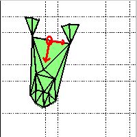
                                                              Figure 1. The alignment points and vectors illustrated on the mesh.

After stereo track, the p shape basis vectors X_k, k=0,...,p are computed using a Singular Value Decomposition (SVD) of the 3D point trajectory X(n). Here, we choose an approach where we can learn the basis vectors on several individuals. First the shapes are aligned for each individual. Figure 1 shows an example mesh with alignment point and vectors on it. The point O is chosen as the middle point of two eyes. The meshes are first translated to point O for compensation of any translation. 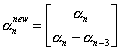Next, the shape is rotated to align the two vectors v₁ and v₂, where v₁ is the vector directing from the point O to the right eye, and v₂ is the vector directing from point O to the tip of the nose. Once all of the shapes are aligned, the neutral shape X₀^u is estimated for each individual u. This is easily accomplished by assigning X₀^u to the shape in the initial frame since the sequences start with the neutral shape of the individual:

                                                                                                                       
Then, the neutral shape is subtracted from the whole trajectory for each individual u. This way, the difference of each expression from the neutral shape is captured:

                                                                                                              
The new shape trajectory X^u(n) is then used to build the following matrix:
                                                

where the subscripts on X denote the individuals, and t denotes the total number of individuals in the training set and Nⁱ denotes the number of frames in the sequence that belongs to the ith individual.  Observe that the neutral-subtracted shapes from each individual is used all together in our calculations. Here we assume that the same expression would result with the same deformation from the neutral shape in different users. Applying Singular Value Decomposition (SVD) on M:
                                                                                                                       
where U and V are two unitary matrices and S is the diagonal matrix of the positive and monotically increasing singular values. The columns of U give the principal movement directions, and we can choose the first p of the columns for p degrees of freedom on the shape. Following this decomposition, we can represent any shape X in terms of the principal movement directions as follows:
                                                                                                                   

Observe that, the neutral shape has a subscript u, which denotes the individual that the mesh belongs to. For any shape X, the shape vector and can be obtained by, 

The stereo tracking procedure produces a shape model that guarantees optimally in approximating the point trajectories computed from stereo tracking (in 
the least squares sense). There are two main functions of the stereo tracking stage: First, the principal movement directions are calculated and used for monocular tracking as long as the user produces a variety of facial expressions that have been exposed to the system during stereo shape learning. Second, the alpha vectors (shape vectors) obtained for the stereo tracking stage acts as training data for support vector machine classification as discussed in the next section.                                                          

3.1.2. Support Vector Machine 

The shape vectors extracted from the stereo tracking data are used in the training set. Each expression is put into one of 5 different expression, i.e.'rigid face shape, opening mouth movement, closing mouth movement, smiling movement, raising eyebrow movement'. Without loss of generality, let us first consider two- class classification problem, i.e. classification between the smiling expression v.s. all other expressions.

Given the representative vectors for the expressions, the optimum classifier has to be obtained using the training data set. The goal is to find a separation function that can be induced from the known data points and generalizes well on the unknown examples. Proposed first by Vapnik, SVM classifier aims to find the optimal differentiating hypersurface between the two classes. In the general case, the optimal hypersurface is the one that not only correctly classifies the data, but also maximizes the margin of the closest data points to the hypersurface.

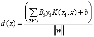
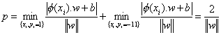
Mathematically, we consider the problem of separating the training set S of points x_i (from Rⁿ) with i = 1,2,…, N. Each data point x_i belongs to either classes and thus is given a label y_i (from {-1,1}). The goal is then to find the optimal hypersurface that separates the two classes. The equation of a hyperplane is given by, (w.f(x))+b=0, where w is the plane normal direction, b is the distance of the plane to the origin and f is the transfer function to map the point to an higher dimensional space. Observe that, the hypersurface transfers to a hyperplane in the high dimensional space. The distance of a point x_i to the hyperplane(w,b) is given by d_i =║f(x_i).w+b║/║w║. The optimal hyperplane is calculated by maximizing the margin, p, i.e. the total distance of two closest points from each class:

The solution of this optimization problem is given by the following optimization problem as discussed in [6][7]:

where K(x_i,x_j) is the inner product of f(x_i)^Tf(x_j) and called the kernel function that satisfies the Mercer’s conditions[6]. Examples of common kernel functions are given in table 1. Once this optimization problem is solved for ß, the support vectors are the data points that have ß_i >0. In other words, support vectors are essentially closest points to the optimal separating hypersurface. A very explanatory description of the support vectors then would be, “the data points that carry the differentiating characteristics between the two classes”. Once we know the support vectors, a new data point is classified as follows:

The distance of the test data from the hypersurface is given as follows:

The most distinguishing property of SVM, is to be able to minimize the structural risk, given as the probability of misclassifying previously unseen data. Besides that, SVMs pack all the relevant information in the training set into a small number of support vectors and use only these vectors to classify the new data. This makes support vectors very appropriate for an application such as expression recognition where we need an automatic way of distinguishing the differentiating characteristics of the expressions.

 Table 1. Some Kernel functions and their mathematical forms

3.2. Testing Stage

Once the training is applied and the optimal differentiating hypersurface between the expressions is determined, the new shape vectors is classified. We have obtained the test data by monocular tracking with different individuals. Since the same face model is used for both stereo and monocular tracking, the obtained shape vectors are comparable for both of the algorithms. In this section, we first describe model based monocular tracking algorithm. Next, the notion of support vector machine is generalized for multi-classes, and the fuzzy probabilistic approach is discussed.

3.2.1 Monocular Tracking 

The algorithm for model-based monocular tracking integrates the standard optical flow algorithm from Lucas and Kanade [21,22] with 
the projection model presented in section 2.In its original form, the optical flow algorithm computes the translational displacement of every point in the image given two successive frames. Each image point is then processed independently by the following optical flow equation:

where I_x and I_y are the image spatial derivatives, and I_t is the image temporal derivative. In the case of model based tracking, each point in the model are linked to each other through the 3D model. In the image plane, each projected point coordinate is a function of the shape vector a(n) and the pose parameters R(n) and T(n). Therefore, the optical flow vector [u v]^T  may be approximated by the product of the Jacobian of [u v]^T with respect to a(n), R(n) and T(n) and the differential shape and pose vector [da(n) dR(n) dT(n)]^T . Let J be the following Jacobian matrix:

replacing u and v in the original Lukas-Kanade equation:

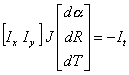
Observe that the tracking output is the vector [da(n) dR(n) dT(n)]  characterizing the differential of pose and deformation between frame n-1 and frame
n. This equation provides a scalar constraint per point on the model. By stacking up all these constrains into a unique linear system, we may solve for the model parameters a(n), R(n) and T(n) all at once. Given any pose of the face, the shape vector a(n) is extracted independently from the pose vectors. This makes the approach much more attractive for a facial expression recognition application.

3.2.2 One to Many Application of SVM and probabilistic approach

    As discussed in 3.1.1, SVM is a two-class classification mechanism. On the other hand, expression recognition is a multi-class classification task. In this section, we propose a method to generalize the two-class classifier for multi-class classification task.

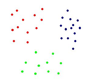
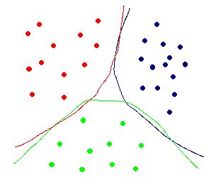
A three class problem is illustrated in figure 2. Using SVM, best differentiating hypersurface can be deduced for each class. This hypersurface is the one that optimally differentiates one class data, from the rest of the data. In other words, a different SVM is trained for each class, to find the hypersurface that distinguishes that particular class from the rest of the data. This is called one to many scheme. Figure 1(a) shows the three classes and 1(b) shows the corresponding hypersurfaces for each classes (same color). 

                                                          (a)                                                                                (b)

            Figure 2. (a) 3 Class of objects in space (b) The corresponding hypersurfaces that differentiate each class from the rest of the data.

Let's now consider a new, test case. The location of the new data is first determined with respect to each hypersurface. For this, the learnt SVM for the particular hypersurface is used to find the distance of the new data to the hypersurface using the distance measure in equation 1. Here, positive distance means that the new data is in the same side with the class that the particular hypersurface distinguishes from the rest. Negative distance means it is at the same side with the rest of the data. Once the distances to all of the hypersurfaces is found, the class that belongs to the maximum hypersurface distance is chosen as the resulting class. Figure 3 gives two particular examples. In 3(a), the new data denoted by the black square, is clearly on the red data side. In 3(b), the new data seems to be not belonging to any classes. In this case, since the data is at the least distance from the green data, it is cassified as the green data.

                                                            (a)                                                                            (b)

                Figure 3. Two examples of classification of test data(black squares) 

While testing each new case, we can assign particular probabilities for each class (expression). Let z_i be the distance of the new data point to the ith class distinguishing hypersurface. The probability that the new data belongs to the ith class is assigned by,

Observe that, some other function can also be used for assigining particular probability. The proposed method is chosen mainly due to the fact that the given function is continuous on  positive and negative values of z_i.

4. Experiments

We used three subjects in our experiments. In the first set of experiments, the training set included totally 240 frames from the stereo sequences of two people. The test data included monocular sequences (monocular sequence is a seperate sequence from the left and right stereo sequences and the person changes his pose in the monocular sequence) of the three subjects. 5 different expressions were used in the experiments: neutral shape,  open mouth, close mouth, smile, raise eyebrow. To differentiate between the open moth and close mouth movements, a velocity term has been added to the shape vector such that:

where the subscript denotes the frame number. In order to observe the effect of different classifiers, we implemented two other classification algorithms for our experiments: Clustering and N-nearest neighbor. In the clustering algorithm, each cluster includes shape vectors for a particular expression. The mean of these training shape vectors give the cluster center. In the test process for a new shape vector, the distances to the cluster centers are compared and the minimum distant cluster center gives the final decision.

N-nearest neighbor algorithm uses a voting strategy to test a new shape data. First, the first N closest training set data points are determined, and each point counts as one vote summing to N votes. The expression with the most votes between these N votes is given as the final decision. 

Table 2 summarizes the results of the experiments in categories of different expressions. Exponential radial basis function (erbf) with standard deviation of  4 was used in this experiment. These results show that All the movements are easy to distinguish except for the neutral shape. The neutral shape is usually confused with the expression that is just before or after itself, which means that many of the false positive detections in neutral shape is due to the transition between the expressions.

Table 2. The response of the system for various expressions

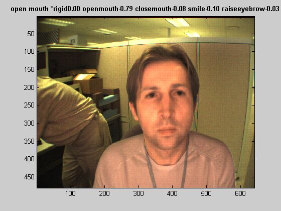
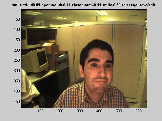
Figure 4 shows examples of some detections and an example of  misclassification. The probabilities assigned to each expression is also given above the pictures. One of the very intuitive improvement of the 3-D system is its robustness to pose changes of the subject. It is observed that the system performs well even with rotations of nearly 90 degree (Figure 4b). The system is able to recognize the expressions even if some of the features are not visible (Figure 4c, the right corner of the mouth and half of the eyebrow are not visible, and the raise eyebrow movement is correctly identified.). In figure 4(a), however, there is a misclassification example. In the following links, you can find the full movies: movie1 and movie2

                                                          (a)                                                                                                               (b)

                                                       (c)                                                                                                                (d)

Figure 4. (a) missclassification example. (b-d) Three correct recognition examples.

Table 3 gives a comparison table between the performances of different methods. The performance criteria is also divided into two groups with test subject in the training set (same person row), and total performance. We observe that SVM has considerable improvement on clustering algorithm, but very slight improvement (practically the same) on N-nearest neighbor algorithm. Observe that the performance of the system for the subjects in the training set is much higher than the subject not in the training set. This is possibly a clue that people have very similar but still different facial expressions.

Table 3. Comparison of performances with different classification methods 

To explain the practically similar performance of N-Nearest algorithm and SVM algorithm, we applied additional analysis on the training set data. In figure 5, we plotted the first four principal component weights of the data. Observe that this is one of the possible ways to be able to plot high dimensional data on 2-D. The first and second principal component extract more information on shape term while the third and fourth components  extract information of the shape velocity term. (The open mouth and smile mouth vectors have similar signatures on the first plot while different signatures on the second plot). We also observe that, there are a number of outliers in the plots. Since SVM is a risk minimization technique, it takes into account the outliers more than the other classifiers and might give some wrong decisions due to this reason.

                                                   (a)                                                                                                                  (b)

Figure 5. The first four principal components of the training set trajectory.

To look further into the performance of the system for subjects out of training set, we ran another set of experiments with only one subject in the training set and three subjects in the test set. The stereo sequence of the person included 130 frames. The results are summarized in table 4. The performance of the system deteriorates with a considerable amount. In addition, the support vector machine classifier performs worse than the other two classifiers. This is mainly due to reduced amount of data in this experiment. We think that there are mainly two reasons for the worse performance: First, the fewer people are contained in the training test, bounding the number of possible personal expressions. Second, there is less data compared to the first experiment, negatively effecting the performance of statistical approaches.

Table 4. Comparison of performances when only one person training set is used.

To look at emotional expressions, we conducted another set of experiments with three expressions: neutral, surprise, happy. The training set included 2 people, and the testing stage included 3 people, 2 of which are the same people with the training set. The results are summarized in table 5. In this experiments, the frames with transition movements between emotions were excluded since it is difficult to label an emotion into those frames. Since the outliers of Figure 5 are excluded in this experiment, the performance of the system becomes as high as %98.

Table 5. Comparison of performances in the tests with three emotional expressions.

Finally, we would like to give a comparison chart with our work and with reported previous work ( the reported work is newer than 1995). Table 6 summarizes the results in different categories. The recognition rate column gives the total rate reported in the paper. The pose change column, gives the amount of rotation that is permitted. The number of expressions gives the number of expressions that has been reported in the experiments. Test/Train subject column reports if the same subject is used in the experiments. The number of data column, gives the amount of test data included in the experiments. 

Table 6. comparison between previously reported facial expression systems (all systems are newer than 1995)

5. Discussion and Conclusion

Facial expression recognition is a necessary application for the future human-computer interaction scenarios. In this study, we propose a new method for robust recognition of facial expressions. The system uses 3-D monocular, markerless face tracker  to extract the shape vector, which is demonstrated to be robust features for classification algorithms. We have shown that 3-D information not only improves the recognition rate, but also brings practical value due to its view independency. There are two main contributions of the paper. First, combination of Support Vector Machines classification with the 3-D tracker based features brings breakthrough facial expression recognition rates. Second, we would like to take the attention of  researchers working on any recognition application (face recognition, expression recognition, gesture recognition) that 3-D information is likely to give better recognition results compared to 2-D. 

There are many possible directions for future investigations. First, we would like to apply another set of experiments with more number of subjects and more number of expressions. Second, we would like to investigate further application of face tracking to face recognition. 

Bibliography & References:

¹ W.W. Bledsoe, " Man-machine facial recognition," Panoramic Research Inc.,Palo Alto, CA, 1966.
² Y. Kaya and K. Kobayashi, " A basic study on human face recognition," in Frontiers of Pattern Recognition, 1972, p. 265.
³ D. DeCarlo and D. Metaxas, " The integration of optical flow and deformable models with aplications to human face shape and motion estimation," Proceedings CVPR'96, pages 231-238,1996.
⁴ P. Eisert and B. Girod, " Analyzing facial expressions for Virtual Conferencing," IEEE Computer Graphics & Applications: Special Issue: Computer Animation for Virtual Humans, vol. 18, no. 5, pp. 70-78, September 1998.
⁵ S.B. Gokturk, J. Bouguet, R. Grzeszczuk, " A Data Driven Model for Monocular Face Tracking," Submitted to International Conference on Computer Vision (ICCV) 2001.
⁶ Vapnik V, The Nature of Statistical Learning Theory, New York, Springer-Verlag, 1995.
⁷ http://www.support-vector.net
⁸ E. Ardizzone, A.Chella, R. Pirrone, " Pose Classification Using Support Vector Machines," Neural Networks, 2000. IJCNN 2000, Proceedings of the IEEE-INNS-ENNS International Joint Conference on, pp. 317 - 322 vol.6
⁹ D. Terzopoulos, and K. Waters, " Analysis and Synthesis of facial image sequences using physical and anatomical models," IEEE Transactions on Pattern Analysis and Machine Intelligencem Volume: 156, pp. 569-579, June 1993.
¹⁰ Xilin Chen, Kwong, S., Yan Lu, "Human facial expression recognition based on learning subspace method ,"IEEE International Conference on Multimedia and Expo, 2000. ICME 2000. Pages: 403 - 406 vol.1 ,2000
¹¹ Mei Wang; Iwai, Y.; Yachida, M, Expression recognition from time-sequential facial images by use of expression change model, Proceedings of Third IEEE International conference on Automatic Face and Gesture Recognition, , Page(s): 324 -329, 1998.
¹² Lien, J.J.; Kanade, T.; Cohn, J.F.; Ching-Chung Li, Automated facial expression recognition based on FACS action units ,  Proceedings of Third IEEE International conference on Automatic Face and Gesture Recognition, Pages: 390 - 395 , 1998.
¹³ Sako, H.; Smith, A.V.W, "Real-time facial expression recognition based on features' positions and dimensions", Proceedings of the 13th International Conference on Pattern Recognition, Volume: 3 , 1996 , Page(s): 643 -648.
¹⁴ Hara, F.; Kobayashi, H, "A face robot able to recognize and produce facial expression ," Proceedings of the 1996 lEEE/RSJ International Conference on Intelligent Robots and Systems '96, IROS 96, Pages: 1600 - 1607 vol.3
¹⁵ Jyh-Yeong Chang; Jia-Lin Chen , "A facial expression recognition system using neural networks ," International Joint Conference on Neural Networks, 1999. IJCNN '99, Pages: 3511 - 3516 vol.5 .
¹⁶ Matsuno, K.; Chil-Woo Lee; Kimura, S.; Tsuji, S. , "Automatic recognition of human facial expressions ,"International Conference on Computer Vision, ICCV'95,Pages: 352 - 359 .
¹⁷ Chandrasiri, N.P.; Min Chul Park; Naemura, T.; Harashima, H. , "Personal facial expression space based on multidimensional scaling for the recognition improvement ," Proceedings of the Fifth International Symposium on Signal Processing and Its Applications, 1999. ISSPA '99.
¹⁸ Hai Hong; Neven, H.; von der Malsburg, C. , "Online facial expression recognition based on personalized galleries ," Proceedings of Third IEEE International conference on Automatic Face and Gesture Recognition, Pages: 354 - 359 , 1998.
¹⁹ Sakaguchi, T.; Morishima, S. , " Face feature extraction from spatial frequency for dynamic expression recognition , " Proceedings of the 13th International Conference on Pattern Recognition, ICPR'96, Volume: 3 , 1996 , Page(s):451 -455.
²⁰ Kobayashi, H.; Tange, K.; Hara, F^. , " Real-time recognition of six basic facial expressions ," Proceedings., 4th IEEE International Workshop on Robot and Human Communication, Pages: 179 - 186 ,1995.
²¹ J.Shi, C. Tomasi, Good features to track, International conference on computer vision and pattern recognition,  CVPR 1994.
²² Lucas, B.D. and Kanade, T., "An iterative image registration technique with an application to stereo vision,"Proc. 7th Int. Conf. on Art. Intell.,1981