The ideas and results contained in this document are part of my thesis, which will be published as a Stanford computer science technical report in June 1999.

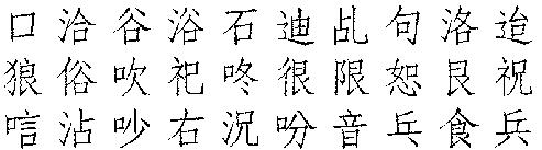
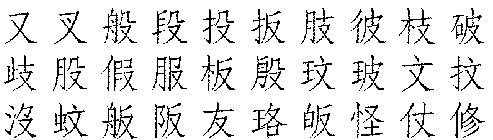
I thank Madirakshi Das from the FOCUS project at University of Massachussetts for the advertisements used in my color database experiments, and Oliver Lorenz for the Chinese characters used in my shape database experiments.

Table of Contents

• Introduction
• The Pattern Problem
• The SEDL Image Retrieval System
  • Overview
    • The Three Phases
    • The Importance of Scale
  • Image Signatures
  • The Scale Estimation Phase
    • The Main Ideas
    • Some Details
    • Results
  • The Initial Placement Phase
    • The Main Ideas
    • Results
  • The Verification and Refinement Phase
    • The Main Ideas
    • Some Details
    • Results
  • Experiments with a Color Database of Product Advertisements
  • Experiments with a Shape Database of Chinese Characters

Introduction

The motivation and setting for my work is content-based image retrieval (CBIR). There are many image retrieval systems that use a global measure of image similarity. By global, I mean that the notion of similarity assumes that all of the information in a database image matches all of the information in the query. A global or complete match distance measure penalizes any information in one image which does not match information in the other image. An example of a complete match distance measure is the L₁ distance between color histograms taken over entire images.

While the assumption of complete matching is convenient and sometimes useful, it is not conducive to building systems that retrieve images which are semantically related to a given query image or drawing. Semantic image similarity, which is what CBIR users will expect and demand, often follows only from a partial match between images as shown in the figure below.

These two images are semantically related because they both contain zebras. This is obviously a case where a partial match distance measure is appropriate. There are no clouds and sky in the right image, and there are no trees in the left image.

If we ever want to obtain semantic similarity from measures of visual similarity, then our notion of visual similarity must allow for partial matching of images. A partial match distance measure is small whenever the image and query contain similar regions, and does not necessarily penalize information in one image that does not match information in the other.

Another important point to be made here is that semantic similarity often follows from only a very small partial match. For example,

The Pattern Problem

The pattern problem is important in image retrieval because its solution may allow users to query a database for images containing a specific item (e.g. object, product logo, machine part, etc.). This is a very common form of query in a text-based system, where, for example, a user may be looking for all articles that mention a specific term.

The main difficultly in efficiently solving a single pattern problem is the combination of partial matching and scaling. Allowing partial matching means that we do not know where in the image to look, and allowing scaling means that we do not know how much of the image to look at. Furthermore, there are many independent (i.e. non-overlapping) places in the image to look for very small scale occurrences of a pattern. In addition to these efficiency difficulties, there is the fundamental issue of how to combine color (shape) information with position information in judging the similarity of two color (shape) patterns.

In the context of database query, the fact that partial match distance measures do not obey the triangle inequality is also an impediment to efficiency. In the example below,

The SEDL Image Retrieval System

Overview

The Three Phases

The purpose of the scale estimation phase is to compute an estimate for the scale at which the pattern may occur within the image. In the example above, the pattern is about 10% of the image. The third column of the first row shows the pattern scaled to reflect the computed estimate. One can see that the estimate in this example is very accurate. The scale estimation phase uses the amounts of colors within the image and query pattern, but not their locations.

The purpose of the initial placement phase is to identify regions in the image that have a similar color histogram to the color histogram of the query. These are promising regions for the pattern occurrence, and will be explored further in the next phase. The size of each candidate region is determined by the scale estimate from the previous phase. There is preprocessing performed so that at query time the system never examines image locations which obviously do not contain the pattern.

During the final verification and refinement phase, the system checks/verifies that the positions of the colors within a promising image region make sense. At this time it also adjusts/refines its guess as to the scale, orientation, and location of the pattern in order to improve a match distance measure that uses the positions of uniform color regions within the query pattern and image. An iterative match improvement process is directed by the region colors since these colors are unchanged by the allowed similarity transformation of pattern region positions. Eventually, the search rectangle settles (SEDLs) on the image region where the system believes that the pattern occurs.

The Importance of Scale

The point here is that a system might falsely conclude that the pattern does not occur within an image because its scale estimate is incorrect. This can happen even when the system has the correct location for the pattern (as shown above).

Image Signatures

For now, one should think of the attribute as color. The A_I are points in a color space, the P_I are points in the image plane, and the W_I are areas in the image. An example is shown below.

In general, the signel (signature element) ((A_I,P_I),W_I) indicates the presence of a region of color A_I with area W_I and centroid P_I. In the above image, we see, for example, that there is yellow (A₄) region at P₄ with area W₄ (perhaps W₄=2% of the total image area), and purple regions at P₁ and P₃ with areas W₁ and W₃, respectively.

The reason that attribute is used instead of color in the above description is that the SEDL framework can also be applied to the shape pattern problem. When this is done, the attribute used by the system is the orientation of ink along curves in an image. In the shape case, the signel ((A_I,P_I),W_I) indicates the presence of a piece of an image curve with length W_I, average orientation A_I, and average position P_I.

Distributions in Attribute x Position space are used by the initial placement and verification phases. Both of these phases use position information. In the color pattern problem setting, the initial placement phase needs to know whether a uniform color region occurs inside or outside of a rectangle. This allows the system to compute the local image color histogram inside of a rectangular region. The verification and refinement phase uses absolute region positions to check that an image area is visually similar to the query (which may not be the case if there is simply a good match between color histograms), and to improve its estimate of the scale, orientation, and location of the pattern occurrence.

The scale estimation phase does not use the positions of the colors within the image. The inputs to the scale estimation phase are distributions of mass in Attribute space, not Attribute x Position space. For example, if the Color x Position distribution of an image notes 10% red at the top of the image and 20% red at the bottom, then the Color distribution notes only that there is 30% red in the image. The input Attribute distribution to the scale estimation phase is obtained by marginalizing out the position information from the Attribute x Position distribution, as in the color example just given.

The Scale Estimation Phase

The Main Ideas

A color signature is a collection of (color,weight) pairs, where the weight of a color is the fraction of image pixels classified as that color. For example the query color signature (Y,u), shows that about u₁=23% of the query is y₁=white, u₂=18% is y₂=dark green, and u₃=17% is y₃=yellow. It is convenient to think of color signatures as discrete distributions of mass/weight in some color space with total weight 1=100%.

In the example above, the query is about 10% of the total database image area. Suppose we scale down the query signature to have total weight 0.10 instead of 1.0, as shown in the above color signature labelled "Scaled Comet Logo Signature". Then all the color mass in the scaled query signature can be matched to similar-color mass in the image signature (90% of the color mass in the image is not needed to perform this match). If we decrease the total weight of the query to less than 0.10, the match does not improve because we already had enough image mass of each query color to match all the query mass when the total was 0.10. If we increase the total weight of the query to more than 0.10, then, the match will get worse because, for example, there will not be enough red and yellow mass in the image to match the red and yellow in the scaled query.

There is a distance measure between discrete distributions of mass called the Earth Mover's Distance (EMD). One can prove that the EMD between the image distribution and the scaled query distribution decreases as the scale parameter c is decreased, and furthermore that this distance becomes constant for all c <= c⁰. This coincides with the intuition given in the previous paragraph. A portion of the graph of EMD versus c for the comet example is shown above, to the right of the color signatures. The value c⁰ is used as an estimate for the scale at which the pattern appears in the image.

In the comet example, the scale estimate is very accurate. If, however, there were a bit more red and yellow in the image than just in the query occurence, then the scale estimate would be a bit too large. This is because "background" red and yellow in the image matches the red and yellow in the query just as well as the red and yellow from the query occurrence. In general, the scale estimation algorithm has the attractive property that the accuracy of the scale estimate is determined by the query color with the least background clutter within the image. The larger this minimum background clutter, the more overestimated the scale. Since there is no background clutter for red and yellow in the comet example, the scale estimate were very accurate, and this is despite the fact that there is a lot of background clutter for white (since there is a lot of white in the image that is not part of the query occurrence). In summary, just one query color with a small amount of background clutter in the image is enough to obtain an accurate scale estimate.

Some Details

The user provides some minimum scale c_min that he/she is interested in finding the pattern. For simplicity of description, assume c⁰ >= c_min. Then initially we know is that c⁰ is somewhere in the interval [c_min,1]. If we check the value of the EMD at the midpoint c_mid of this interval, and, as in the example above, it is greater than the EMD at c_min, then we know that c⁰ is somewhere in the smaller interval [c_min,c_mid] (since the EMD decreases as c decreases). By checking the value of the EMD at the midpoint of the interval in which we are sure that c⁰ occurs, we can keep reducing the size of this interval (shown as a thick line segment in the graphs above) until it becomes smaller than some user-specified precision for the scale estimate.

Although the EMD versus c curve must become constant for c small enough, this constant value may be large. This can happen, for example, if a substantial portion of the query pattern is red, but there is no color in the image which is at all similar to red. When the EMD curve flattens out at a large EMD value, the system asserts that the pattern does not occur within the image, and it does not perform the the initial placement and refinement stages.

Results

Some results from the scale estimation phase are shown below. To the right of each image is the pattern scaled according to the estimate.

The scale estimate is fairly accurate in all of these examples, although it is a little too small for all but the final tide example. The scale is overestimated in the tide example because the pattern appears twice within the image. Since the scale estimation phase uses only the amounts of colors, and not their positions within the image, the algorithm cannot tell the difference between one pattern occurrence of scale c and two pattern occurrences of scales d and e, where c=d+e.

More results for the scale estimation are shown below.

As above, the scale estimate is fairly accurate in all of these examples. The estimate is a little too small for all but the final misty example in which the pattern occurs twice. In this example, the scale estimate is close to the sum of the scales of the two pattern occurrences.

The Initial Placement Phase

The Main Ideas

The flow variable f⁰_ij is the amount of color j from the scaled pattern that matches color i in the image. Using the flow F⁰, we can compute the probability or confidence q_i that an image pixel of color i is part of the pattern occurrence, assuming that the pattern does indeed occur within the image.

Assuming a good scale estimate, the sum_jf⁰_ij over all pattern colors j is a good estimate of the amount of image color i that is part of the pattern occurrence within the image. If this sum is equal to the total amount w_i of color i within the image, then one is 100% confident that a random image pixel of color i is part of the pattern occurrence (assuming that the pattern is present in the image). In general, the probability q_i that a random image pixel of color i is part of the pattern occurrence is

The confidence q_i is inversely related to the amount of backgound clutter of color i within the image. Here backgound clutter refers to all image pixels which are not part of the pattern occurence.

An example illustrating the confidence q_i is given below.

Yellow is basically a 100% confidence color since all the yellow in the image is needed to match yellow in the scaled query. Purple is also a high confidence color. About 90% of the purple in the image is matched to purple in the scaled query. The confidence for purple is not 100% because the pattern does not include all the purple on the ziploc box, and the pattern is slightly underestimated in scale. White and black are low confidence colors. Although the white on the ziploc box within the image is needed to match white in the scaled query, there is a lot of other white in the image (the writings "I will keep my sandwich fresh" and "Ziploc has the lock on freshness", the chalk next to the ziploc box, and the white on the ziploc box that is not part of the pattern). The black in the image is not needed to match any color in the pattern.

The initial placement phase compares the local image color distribution inside of rectangular image regions to the color distribution of the pattern. The main idea here is that we only need to check image locations of high confidence colors. In the above ziploc example, we never need to examine a region in the upper part of the ziploc advertisement since there are only low confidence colors present (black and white). The search for image regions with similar color signature to the query is thus directed (the D in SEDL) by the high confidence colors. The size of the rectangular regions examined is determined by the scale estimate c⁰. The image signature is preprocessed in order to answer range search questions at query time : what are all the image regions inside a given rectangular area? This range search capability allows the system to compute the local image color signature inside of a rectangle.

Results

In each of these examples, at least one of the initial placements significantly overlaps the pattern occurence. In the final tide example, where the scale is overestimated, one of the initial placements contains both occurrences of the pattern.

More results from the initial placement phase are shown below.

As above, at least one of the initial placements significantly overlaps the pattern occurence in all these examples. In fact, one of the initial placements in the taco bell example is near perfect.

The Verification and Refinement Phase

The Main Ideas

The figure below illustrates the main ideas in this phase.

In the left column, there is a pattern above an image which contains that pattern at a different scale and orientation. In the center column, I have shown the pattern and image signatures in Color x Position space. In these signatures, only the locations and colors of the regions are shown, not their areas. For example, the three blue circles in the pattern signature represent the three blue letters in the pattern. The occurrence of the pattern in the image gives rise to a similar set of signels in the image signature. There is a similarity transformation g=g^* of the pattern regions that aligns the regions in the pattern with regions of the same color in the image. Our goal is to find that optimal transformation g=g^*. The main idea is to start from a transformation g⁰ determined by the scale estimation and initial placement phases (see the right column), and iteratively refine the estimate for the pattern scale, orientation, and location until the match stops improving. In this example, only the pattern orientation needs to be adjusted, since the location and scale are already correct.

Some Details

Here is the signature for the pattern in the above example.

We assume that both signatures are normalized to have total weight 1(=100% of an image).

We shall define a distance between signatures in Attribute x Position space based on a distance between signels in Attribute x Position space. For the color case, the distance in Color x Position space measures the overall distance between two regions with possibly different colors and locations. We use a linear combination of attribute and position distance :

where the constant K trades off the importance of distance in attribute space with the distance in the image plane (and accounts for the possibly different orders of magnitude returned by the individual attribute and position distance functions). In the color case, d_attr(A_I,B_J) is the Euclidean distance between colors A_I and B_J represented in CIE-Lab space coordinates. In the shape case, d_attr(A_I,B_J) is the distance in radians between two angles A_I and B_J.

The distance between the image signature X and the pattern signature Y is given by

Let us explain this formula in terms of the color case. For the moment, ignore the minimization and just consider the summation. Each pattern region J is matched to some image region f(J) (in {1,...,M}). The distance between these regions in Color x Position space is computed and weighted by the area of pattern region J. These weighted region-region distances are summed over all pattern regions. The signature distance D_G(Y,X) allows for a transformation g of the query region positions (taken from some given set of transformations G), and calls for the minimum weighted sum of region-region distances over all possible pairs of correspondences and transformations.

At least a locally optimal transformation can be computed by alternately computing the best set of correspondences for a given transformation, then the best transformation for the previously computed correspondences, then the best set of correspondences for the previously computed transformation, and so on. The summation in the formula for D_G(Y,X) gives a value for every (correspondence set f, transformation g) pair, and thus defines a surface over the space FxG of all such pairs. The alternation strategy gives a way to follow a path downhill along this surface. The job of the scale estimation and initial placement phases is to define the initial transformation g⁰ to be close to the globally optimal transformation g^* so that our iteration converges to this globally optimal transformation or to a transformation which is nearly optimal.

The search for the minimum D_G(Y,X) is directed by the colors of the regions since these are unchanged by transformations g in G. The system will not match two regions which are close together unless their colors are similar. As in the initial placement phase, directed should be compared with exhaustive. Here, the search for the optimal transformation does not simply try a discrete sampling of all transformations in some neighborhood of the initial transformation. The verification and refinement stage uses the image data, in particular the colors and layouts of the image regions to adjust/refine its estimate of the pattern scale, orientation, and location.

Results

Some results from the verification phase are shown below. The red rectangle indicates the scale, orientation, and location where SEDL believes that the pattern occurs.

In general, these results are excellent. The localization of the pattern in the breathe right, jello, reynolds, and clorox, and cornpops advertisements is near perfect. The orientation is slightly off in the pert example in the first row, third column. The system makes a mistake in its search for the pert logo within the pert advertisement in the second row, third column. In the tide example in row three, column two, the scale is decreased from the initial overestimate, but the rectangle settles between the two pattern occurrences.

More results from the verification phase are shown below.

In the first two misty advertisements in row one, the system was searching for the entire cigarette box, but ended up aligning the final rectangle to a major portion of the pattern occurence (the stripes on the box). In the third misty example in row one, SEDL finds one of the two pattern occurrences. In the scholl's example in row two, column three, SEDL finds one of the four pattern occurrences (despite an initial overestimate in scale). The postion and orientation in the taco bell example should be better. The ziploc and casting results are near perfect. The system never quite recovered from the initial scale overestimate in the misty advertisement in row three, column two; the final rectangle, however, contains both occurrences of the pattern.

Experiments with a Color Database of Product Advertisements

We use four initial placements in our experiments, although two initial placements usually suffices (as shown in the results for the initial placement phase).

For 20 return images, SEDL achieved a recall rate of 78% over the 25 queries. This means that 78% of all advertisements that should have been retrieved over all 25 queries were retrieved in the top 20. Of course, a query result with the three breathe right advertisements returned as 1st, 2nd, and 3rd is more precise a result than if the three are returned 1st, 5th, and 20th, which is more precise than if the three are returned 18th, 19th, and 20th. The precision is a number between 0 and 1 which measures how close to perfect ranks the correctly returned images occurred, where 1 is perfect precision. The precision of SEDL over all 25 queries is 0.88. With 20 return images, SEDL achieved high recall and high precision. The average time for one query is T_avg=40 seconds, which is about 0.1 seconds per query-image comparison.

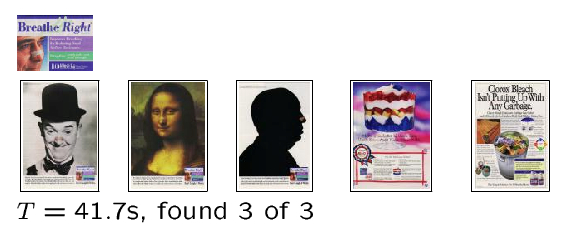
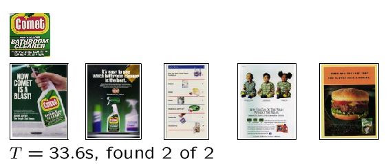
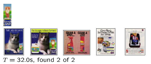
Some SEDL query results are shown below. The query time and the number of correct advertisements returned in the top twenty are shown below each result. For the first five queries, SEDL achieved perfect recall and precision.

The three breathe right ads are returned 1st, 2nd, and 3rd.

The two comet ads are returned 1st and 2nd.

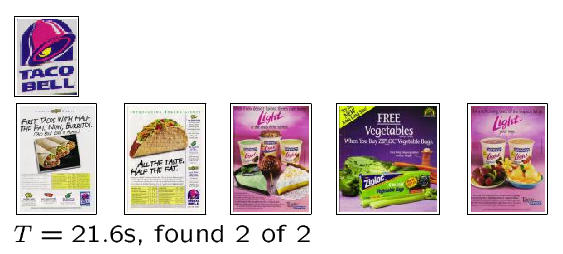
The two taco bell ads are returned 1st and 2nd.

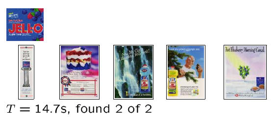
The two jello ads are returned 1st and 2nd.

The two fresh step ads are returned 1st and 2nd.

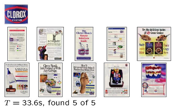
The clorox query result is perfect recall, but not perfect precision.

The five clorox ads are returned 1st, 3rd, 4th, 7th, and 8th.

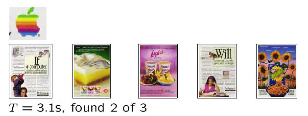
The Apple query result is neither perfect recall nor perfect precision.

One of the three Apple ads is not returned in the top twenty. The remaining two Apple ads are returned 1st and 4th.

Experiments with a Shape Database of Chinese Characters

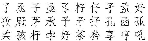
The same code run on the color advertisement database is run on the shape Chinese character database, but with a different interpretation of attribute. In the shape case, the attribute is the orientation of the ink along image curves.

The signature creation process is not performed directly on the bitmaps, but rather on the medial axis for the database characters since this makes it clearer exactly what are the image curves. The medial axis curves are divided into (relatively) small, equal length pieces. Each curve piece gives rise to a signel ((A_avg,P_avg),L) in the Orientation x Position image signature, where A_avg is the average orientation along the curve piece, P_avg is the average position along the curve piece, and L is the length of the piece.

The set of allowable transformations consists of scalings and translations. Since rotations are not allowed, the orientation of ink on the page guides or directs the search process. The system will not match ink at the same location on the page unless the orientations are relatively close. Two initial placements are used. The average query time over 15 different queries is T_avg=95.7 seconds, which is about 0.05 seconds per query-image comparison.

The results of a few queries are shown below. In each case, the query pattern is shown on the left, and the top 30 return images are shown on the right. We also show where SEDL believes the pattern occurs in a small sample of the returned images.

The ideas and results contained in this document are part of my thesis, which will be published as a Stanford computer science technical report in June 1999.

S. Cohen. Finding Color and Shape Patterns in Images. Thesis Technical Report STAN-CS-TR-99-?. To be published June 1999.

Email comments to scohen@cs.stanford.edu.